Developing a new Analysis for BASTet
BASTet provides developers with two easy ways to integrate new analyses. First, the simplest and most basic solution is to wrap analysis functions using either the @bastet_analysis Python decorator or by explicitly wrapping a function via wrapped funct = analysis generic.from function(my function). Second, to easily share and fully integrate an analysis with BASTet, we then create a new class that inherits from BASTet’s base analysis interface class
Wrapping a function: The quick-and-dirty way
Sometimes developers just want to debug some analysis function or experiment with different variants of a code. At the same time, we want to be able to track the results of these kind of experiments in a simple fashion. The omsi.analysis.generic() provides us with such a quick-and-dirty solution. We say quick-and-dirty because it sacrifices some generality and features in favor for a very simple process.
Using the omsi.analysis.generic.analysis_generic.from_function() or omsi.analysis.generic.bastet_analysis() decorator, we can easily construct a generic omsi.analysis.base.analysis_base instance container object for a given function. We can then use this container object to execute our function, while tracking its provenance as well as save the results to file as we would with any other analysis object. This approach allows us to easily track, record, safe, share and reproduce code experiments with only minimal extra effort needed. Here we briefly outline the two main options to do this.
NOTE: Wrapping functions directly is not recommended for production workflows but is intended for development and debugging purposes only. This mechanism relies on that the library does the right thing in automatically determining input parameters, outputs, and their types and that we can handle all those types in the end-to-end process, from definition to storage. We do our best to make this mechanism work with a broad set of cases but we do not guarantee that the simple wrapping always work.
Option 1: Explicitly track specific excutions of a function
Instead of calling our analysis function f() directly, we create an instance of omsi.analysis.generic.analysis_generic() via g = analysis_generic.from_function(f) which we then use instead of our function. To execute our function we can now either call g.execute(...) as usual or treat g as a function and call it directly g(...)
1 2 3 4 5 6 7 8 9 10 11 | import numpy as np
from omsi.analysis.generic import analysis_generic
# Define some example function we want to wrap to track results
def mysum(a):
return np.sum(a)
# Create an analysis object for our function
g = analysis_generic.from_function(mysum)
g['a'] = np.arange(10) # We can set all parameters prior to executing the function
g.execute() # This is the same as: g(np.arange(10))
|
See omsi.analysis.generic.analysis_generic.from_function() for further details on additional optional inputs of the wrapping, e.g., to specify additional information about inputs and outputs.
Option 2: Implicitly track the last execution of a function
If we are only interested in recording the last execution of our function, then we can alternatively wrap our function directly using the @bastet_analysis decorator. The main difference between the two approaches is that using the decorator we only record the last execution of our function, while using the explicit approach of option 1, we can create as many wrapped instances of our functions as we want and track the execution of each independently.
1 2 3 4 5 6 7 8 9 10 11 12 13 14 15 16 17 | import numpy as np
from omsi.shared.log import log_helper
log_helper.set_log_level('DEBUG')
from omsi.analysis.generic import bastet_analysis
# Define some example function and wrap it
@bastet_analysis
def mysum(a):
"""Our own sum function"""
return np.sum(a)
# mysum['a'] = np.arange(10)
# As with the any wrapped function we can delay execution and set
# parameters before we actuall run the analysis
# Execute the analysis
res = mysum(a=np.arange(10)) # Or we can set parameters and execute in the same call
|
See omsi.analysis.generic.bastet_analysis() for further details on additional optional inputs of the wrapping, e.g., to specify additional information about inputs and outputs.
Example 1: Defining and using wrapped functions
The code example shown below illustrates the “wrapping” of a simple example function mysum(a), which simply uses numpy.sum to compute the sum of objects in an array. (NOTE: We could naturally also use numpy.sum directly, we use mysum(a) mainly to illustrate that this approach also works wit functions defined in the interpreter.)
1 2 3 4 5 6 7 8 9 10 11 12 13 14 15 16 17 18 19 20 21 22 23 24 25 26 27 28 29 30 31 32 33 34 35 36 37 | import numpy as np
from omsi.shared.log import log_helper
log_helper.set_log_level('INFO')
from omsi.analysis.generic import analysis_generic
from omsi.dataformat.omsi_file.main_file import omsi_file
# Define some example function we want to wrap to track results
def mysum(a):
return np.sum(a)
# Create an analysis object for our function
g = analysis_generic.from_function(mysum)
# Execute the analysis
res = g.execute(a=np.arange(10))
log_helper.log_var(__name__, res=res) # Logging the result
# Save the analysis to file
f = omsi_file('autowrap_test.h5', 'a')
e = f.create_experiment()
exp_index = e.get_experiment_index()
ana_obj, ana_index = e.create_analysis(g)
# Close the file
f.flush()
del f
# Restore the analysis from file
f = omsi_file('autowrap_test.h5', 'a')
e = f.get_experiment(exp_index)
a = e.get_analysis(ana_index)
g2 = a.restore_analysis()
res2 = g2.execute()
log_helper.log_var(__name__, res2=res2) # Logging the result
if res == res2:
log_helper.info(__name__, "CONGRATULATIONS---The results matched")
else:
log_helper.error(__name__, "SORRY---The results did not match")
|
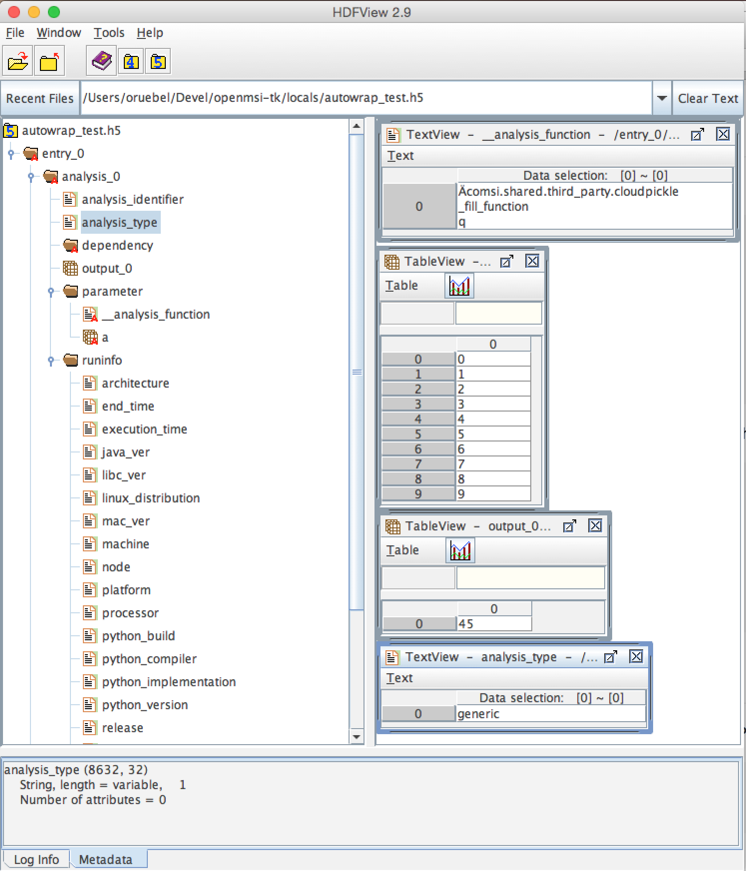
When we run our script, we can see that we were able to successfully capture the execution of our function and recreate the analysis from file.
1 2 3 4 | machine:dir username$ python autowrap_function.py
2015-09-29 15:21:32,729 - __main__ - INFO - res = 45
2015-09-29 15:21:32,778 - __main__ - INFO - res2 = 45
2015-09-29 15:21:32,778 - __main__ - INFO - CONGRATULATIONS---The results matched
|
The figure below shows a view of the file generated by our wrapped function execution example shown above.
Note, we can use the wrapped function objects as usual in an analysis workflow to combine our functions with other analyses. For example, the simple example shown below shows how we can quickly define a simple filter to set all intensities that are less than 10 to a value of 0 before executing an analysis. We here first execute global peak finding to reduce the data, than apply a simple wrapped filter function to filter the data values, and then compute NMF on the filtered data.
1 2 3 4 5 6 7 8 9 10 11 12 13 14 15 16 17 18 19 20 21 22 23 24 25 26 27 28 | from omsi.dataformat.omsi_file import *
from omsi.analysis.findpeaks.omsi_findpeaks_global import omsi_findpeaks_global
from omsi.analysis.multivariate_stats.omsi_nmf import omsi_nmf
from omsi.analysis.generic import analysis_generic
import numpy as np
f = omsi_file('/Users/oruebel/Devel/openmsi-data/msidata/20120711_Brain.h5' , 'r')
d = f.get_experiment(0).get_msidata(0)
# Specify the analysis workflow
a1 = omsi_findpeaks_global()
a1['msidata'] = d
a1['mzdata'] = d.mz
# Wrap a simple function to filter all peaks with less than 10 counts
def f(a):
a[a<10] = 0
return a
a2 = analysis_generic.from_function(f)
a2['a'] = a1['peak_cube'] # Use the peak_cube from a1 as input for the filter
# Create an NMF for the filtered data
a3 = omsi_nmf()
a3['msidata'] = a2['output_0'] # Make the output of our analysis the input of the NMF
a3['numIter'] = 2
# Run our simple workflow, i.e.,: peak_finder --> our_filter --> nmf
a3.execute_recursive()
|
By default, the outputs are named and numbered using the schema output_#, i.e., in the above example we used a2['output_0'] to access the output our wrapped function. To define user-defined names for the outputs of a wrapped function we can simply provide a list of strings to the input parameter output_names of the analysis_generic.from_function(...).
Writing a new analysis class for BASTet – Part 1: Overview
The OpenMSI Toolkit includes a basic template for implementing new analyses as part of OpenMSI. The template is located in omsi.templates.omsi_analysis_template.py. The template provides step-by-step instructions on how to implement a new analysis. Simply search top-to-bottom for EDIT_ME markers to find locations that need to be edited and what changes need to be made.
The implementation of a new analysis is divided into three main steps. We here provide a brief overview of these steps. A detailed walk-through the required implementation is provided in the following sections.
Step 1) Basic integration of your analysis with OpenMSI (Required)
The basic integration is simple and should requires only minimal additional effort. The basic integration with the OpenMSI provides:
- full integration of the analysis with the OpenMSI file format and API
- full support for OpenMSI’s data provenance capabilities
- full integration with analysis drivers (e.g, the command line driver) enabling direct execution of the analysis with automatic handling of user input specification, help, etc.
- basic integration of the analysis with the website, in that a user will be able to browse the analysis in the online file browser. The basic integration automatically provides full support for the
qmetadataandqcubeURL data access patterns. The basic integration provides limited support for theqslice,qspectrum, andqmzpatterns, in that it automatically exposes all dependencies of the analysis that support these patterns but it does not expose the data of the analysis itself. This is part of step 2.
Step 2) Integrating your analysis with the OpenMSI web-based viewer (Recommended)
Once the basic integration is complete, you may want integrate your analysis fully with the OpenMSI online viewer, in order to make your analysis easily accesible to the OpenMSI user community. This step requires the implementation of the qslice, qspectrum, and qmz URL patterns for the analysis. This step completes the integration with the OpenMSI framework itself.
Step 3) Making your analysis self-sufficient (Recommended)
This step makes your analysis “self-sufficient” in that it allows you to execute your analysis from the command-line. This step is usually very simple as we can just use BASTet’s integrated analysis driver to do the job for us.
Some important features of analysis_base
omsi.analysis.analysis_base is the base class for all omsi analysis functionality. The class provides a large set of functionality designed to facilitate i) storage of analysis data in the omsi HDF5 file format and ii) integration of new analysis capabilities with the OpenMSI web API and the OpenMSI web-based viewer (see Viewer functions below for details), iii) support for data provenance, and iv) in combination with the omsi_analysis_driver module enable the direct execution of analysis, e.g, from the command line
Slicing
analysis_base implements basic slicing to access data stored in the main member variables. By default the data is retrieved from __data_list by the __getitem__(key) function, which implements the [..] operator, i.e., the functions returns __data_list[key][‘data’]. The key is a string indicating the name of the paramter to be retrieved. If the key is not found in the __data_list then the function will try to retrieve the data from __parameter_list instead. By adding “parameter/key” or “dependency/key” one may also explicitly retrieve values from the __parameter_list and __dependency_list.
Important Member Variables
analysis_identifierdefines the name for the analysis used as key in search operations.__data_listdefines a list ofomsi.analysis.analysis_data.analysis_dataobjects to be written to the HDF5 file. Derived classes need to add all data that should be saved for the analysis in the omsi HDF5 file to this dictionary. Seeomsi.analysis.analysis_datafor details.parametersList ofparameter_datato be written to the HDF5 file. Derived classes need to add all parameter data that should be saved for the analysis in the omsi HDF5 file to this dictionary using the providedadd_parameter(...)function. Seeomsi.analysis.analysis_dataandadd_parameter(..)function ofanalysis_basefor details.data_namesis a list of strings of all names of analysis output datasets. These are the target names for __data_list. NOTE Names of parameters specified inparametersanddata_namesshould be distinct.
I/O functions
These functions can be optionally overwritten to control how the analysis data should be written/read from the omsi HDF5 file. Default implementations are provided here, which should be sufficient for most cases.
write_analysis_dataBy default all data is written byomsi.dataformat.omsi_file.analysis.omsi_file_analysis. By implementing this function we can implement the write for the main data (i.e., what is stored in self.__data_list) ourselves. In practice (at least in the serial case) this should not be needed. However, overwriting the function can be useful when implementing an analysis using MPI and we want to avoid gathering the data on rank the root rank (usually rank 0).add_custom_data_to_omsi_file: The default implementation is empty as the default data write is managed by the omsi_file_experiment.create_analysis() function. Overwrite this function, in case that the analysis needs to write data to the HDF5 omsi file beyond what the defualt omsi data API does.read_from_omsi_file: The default implementation tries to reconstruct the original data as far as possible, however, in particular in case that a custom add_custom_data_to_omsi_file funtion has been implemented, the default implementation may not be sufficien. The default implementation reconstructs: i) analysis_identifier and reads all custom data into ii)__data_list. Note, an error will be raised in case that the analysis type specified in the HDF5 file does not match the analysis type specified by get_analysis_type(). This function can be optionally overwritten to implement a custom data read.
Web API Functions
Several convenient functions are used to allow the OpenMSI online viewer to interact with the analysis and to visualize it. The default implementations provided here simply indicate that the analysis does not support the data access operations required by the online viewer. Overwrite these functions in the derived analysis classes in order to interface them with the viewer. All viewer-related functions start with v\_... .
NOTE: the default implementation of the viewer functions defined in analysis_base are designed to take care of the common requirement for providing viewer access to data from all depencies of an analysis. In many cases, the default implementation is often sill called at the end of custom viewer functions.
NOTE: The viewer functions typically support a viewerOption parameter. viewerOption=0 is expected to refer to the analysis itself.
v_qslice: Retrieve/compute data slices as requested via qslice URL requests. The corrsponding view of the DJANGO data access server already translates all input parameters and takes care of generating images/plots if needed. This function is only responsible for retrieving the data.v_qspectrum: Retrieve/compute spectra as requested via qspectrum URL requests. The corrsponding view of the DJANGO data access server already translates all input parameters and takes care of generating images/plots if needed. This function is only responsible for retrieving the data.v_qmz: Define the m/z axes for image slices and spectra as requested by qspectrum URL requests.v_qspectrum_viewer_options: Define a list of strings, describing the different viewer options available for the analysis for qspectrum requests (i.e.,v_qspectrum). This feature allows the analysis developer to define multiple different visualization modes for the analysis. For example, when performing a data rediction (e.g., PCA or NMF) one may want to show the raw spectra or the loadings vector of the projection in the spectrum view (v_qspectrum). By providing different viewer options we allow the user to decide which option they are most interested in.v_qslice_viewer_options: Define a list of strings, describing the different viewer options available for the analysis for qslice requests (i.e.,v_qslice). This feature allows the analysis developer to define multiple different visualization modes for the analysis. For example, when performing a data rediction (e.g., PCA or NMF) one may want to show the raw spectra or the loadings vector of the projection in the spectrum view (v_qspectrum). By providing different viewer options we allow the user to decide which option they are most interested in.
Executing, saving, and restoring an analysis object
Using the command-line driver we can directly execute analysis as follows:
python omsi/analysis/omsi_analysis_driver <analysis_module_class> <analysis_parameters>
E.g. to execute a non-negative matrix factorization (NMF) using the omsi.analysis.multivariate_stats.omsi_nmf module we can simply:
python omsi/analysis/omsi_analysis_driver.py multivariate_stats/omsi_nmf.py
    --msidata "test_brain_convert.h5:/entry_0/data_0"
    --save "test_ana_save.h5"
Any analysis based on the infrastructure provided by analysis_base is fully integrated with OpenMSI file API provided by``omsi.dataformat.omsi_file``. This means the analysis can be directly saved to an OMSI HDF5 file and the saved analysis can be restored from file. In OMSI files, analyses are generally associated with experiments, so that we use the omsi.dataformat.omsi_file.omsi_file_experiment API here.
1 2 3 4 5 6 7 8 9 10 11 12 13 14 15 16 17 18 19 20 21 22 23 24 25 26 27 28 29 30 31 32 33 34 35 36 37 38 39 40 41 42 43 44 45 46 47 48 49 50 51 52 53 54 55 56 57 58 | # Open the MSI file and get the desired experiment
from omsi.dataformat.omsi_file import *
f = omsi_file( filename, 'a' )
e = f.get_experiment(0)
# Execute the analysis
d = e.get_msidata(0)
a = omsi_myanalysis()
a.execute(msidata=d, integration_width=10, msidata_dependency=d)
# Save the analysis object.
analysis_object , analysis_index = exp.create_analysis( a )
# This single line is sufficient to store the complete analysis to the omsi file.
# By default the call will block until the write is complete. Setting the
# parameter flushIO=False enables buffered write, so that the call will
# return once all data write operations have been scheduled. Here we get
# an omsi.dataformat.omsi_file.omsi_file_analysis
# object for management of the data stored in HDF5 and the integer index of the analysis.
# To restore an analysis from file, i.e., read all the analysis data from file
# and store it in a corresponding analysis object we can do the following.
# Similar to the read_from_omsi_file(...) function of analysis_base
# mentioned below, we can decide via parameter settings of the function,
# which portions of the analysis should be loaded into memory
a2 = analysis_object.restore_analysis()
# If we want to now re-execute the same analysis we can simply call
a2.execute()
# If we want to rerun the analysis but change one or more parameter settings,
# then we can simply change those parameters when calling the execute function
d2 = e.get_msidata(1) # Get another MSI dataset
a2.execute(msidata=d2) # Execute the analysis on the new MSI dataset
# The omsi_file_analysis class also provides a convenient function that allows us
# to recreate, i.e., restore and run the analysis, in a single function call
a3 = analysis_object.recreate_analysis()
# The recreate_analysis(...) function supports additional keyword arguments
# which will be passed to the execute(...) call of the analysis, so that we
# can change parameter settings for the analysis also when using the
# recreate analysis call.
# If we know the type of analysis object (which we can also get from file), then we
# naturally also restore the analysis from file ourselves via
a4 = omsi_myanalysis().read_from_omsi_file(analysisGroup=analysis_object, \
load_data=True, \
load_parameters=True,\
load_runtime_data=True, \
dependencies_omsi_format=True )
# By setting load_data and/or load_parameters to False, we create h5py instead of
# numpy objects, avoiding the actual load of the data. CAUTION: To avoid the accidental
# overwrite of data we recommend to use load_data and load_parameters as False only
# when the file has been opened in read-only mode 'r'.
# Rerunning the same analysis again
a4.execute()
|
Writing a new analysis class for BASTet – Part 2: Analysis Template
In this section we describe the basic development of a new analysis using the analysis template provided by BASTet.
Step 1) Basic integration
The simple steps outlined below provide you now with full integration of your analysis with the OpenMSI file format and API and full support for OpenMSI’s data provenance capabilities. It also provides basic integration of your analysis with the OpenMSI website, in that a user will be able to browse your analysis in the online file browser. The basic integration also automatically provides full support for the qmetadata and qcube URL data access patterns, so that you can start to program against your analysis remotely. The basic integration provides limited support for the qslice, qspectrum, and qmz patterns, in that it automatically exposes all dependencies of the analysis that support these patterns but it does not expose the data of your analysis itself. This is part of step 2. Once you have completed the basic integation yout final analysis code should look something like this:
1 2 3 4 5 6 7 8 9 10 11 12 13 14 15 16 17 18 19 20 21 22 23 24 25 26 27 28 29 30 31 32 33 34 35 36 37 38 39 40 41 42 43 44 45 46 47 48 49 50 51 52 53 54 55 56 57 58 59 60 61 62 63 64 | class omsi_mypeakfinder(analysis_base) :
def __init__(self, name_key="undefined"):
"""Initalize the basic data members"""
super(omsi_mypeakfinder,self).__init__()
self.analysis_identifier = name_key
# Define the names of the outputs generated by the analysis
self.data_names = [ 'peak_cube' , 'peak_mz' ]
# Define the input parameters of the analysis
dtypes = self.get_default_dtypes()
groups = self.get_default_parameter_groups()
self.add_parameter(name='msidata',
help='The MSI dataset to be analyzed',
dtype=dtypes['ndarray'],
group=groups['input'],
required=True)
self.add_parameter(name='mzdata',
help='The m/z values for the spectra of the MSI dataset',
dtype=dtypes['ndarray'],
group=groups['input'],
required=True)
self.add_parameter(name='integration_width',
help='The window over which peaks should be integrated',
dtype=float,
default=0.1,
group=groups['settings'],
required=True)
self.add_parameter(name='peakheight',
help='Peak height parameter',
dtype=int,
default=2,
group=groups['settings'],
required=True)
def execute_analysis(self) :
"""..."""
# Copy parameters to local variables. This is purely for convenience and is not mandatory.
# NOTE: Input parameters are automatically record (i.e., we don't need to to anything special.
msidata = self['msidata']
mzdata = self['mzdata']
integration_width = self['integration_width']
peakheight = self['peakheight']
# Implementation of my peakfinding algorithm
...
# Return the result.
# NOTE: We need to return the output in the order we specified them in self.data_names
# NOTE: The outputs will be automatically recorded (i.e., we don't need to anything special).
return peakCube, peakMZ
self['peak_cube'] = peakCube
...
# Defining a main function is optional. However, allowing a user to directly execute your analysis
# from the command line is simple, as we can easily reuse the command-line driver module
if __name__ == "__main__":
from omsi.analysis.omsi_analysis_driver import cl_analysis_driver
cl_analysis_driver(analysis_class=omsi_mypeakfinder).main()
|
1.1 Creating a new analysis skeleton
- Copy the analysis template to the appropriate location where your analysis should live (NOTE: The analysis template may have been updated since this documentation was written). Any new analysis should be located in a submodule of the
omsi.analysis.module. E.g., if you implement a new peak finding algorithm, it should be placed in omsi/analysis/findpeaks. For example:
cp omsi/templates/omsi_analysis_template.py openmsi-tk/omsi/analysis/findpeaks/omsi_mypeakfinder.py
- Replace all occurrences of
omsi_analysis_templatein the file with the name of your analysis class, e.g, omsi_mypeakfinder. You can do this easily using “Replace All” feature of most text editors. or on most Unix systems (e.g, Linux or MacOS) on the commandline via:
cd openmsi-tk/omsi/analysis/findpeaks
sed -i.bak 's/omsi_analysis_template/omsi_mypeakfinder/' omsi_mypeakfinder.py
rm omsi_mypeakfinder.py.bak
- Add your analysis to the
__init__.pyfile of the python module where your analysis lives. In the__init__.pyfile you need to add the name of your analysis class to theall__list and add a an import of your class, e.g,from omsi_mypeakfinder import *. For example:
1 2 3 4 | all__ = [ "omsi_mypeakfinder", "omsi_findpeaks_global" , ...]
from omsi_findpeaks_global import *
from omsi_findpeaks_local import *
...
|
- The analysis template contains documentation on how to implement a new analysis. Simply search for EDIT_ME to locate where you should add code and descriptions of what code to add.
1.2 Specifying analysis inputs and outputs
In the __init__ function specify the names of the input parameters of your analysis as well as the names of the output data generated by your analysis. Note, the __init__ function should have a signature that allows us to instantiate the analysis without having to provide any inputs. E.g.,
1 2 3 4 5 6 7 8 9 10 11 12 13 14 15 16 17 18 19 20 21 22 23 24 25 26 27 28 29 30 31 32 33 34 35 36 37 | def __init__(self, name_key="undefined"):
"""Initalize the basic data members"""
super(omsi_mypeakfinder,self).__init__()
self.analysis_identifier = name_key
# Define the names of the outputs
self.data_names = ['peak_cube', 'peak_mz']
# Define the input parameters
dtypes = self.get_default_dtypes() # List of default data types. Build-in types are
# available as well but can be safely used directly as well
groups = self.get_default_parameter_groups() # List of default groups to organize parameters. We suggest
# to use the 'input' group for all input data to be analyzed
# as this will make the integration with OpenMSI easier
self.add_parameter(name='msidata',
help='The MSI dataset to be analyzed',
dtype=dtypes['ndarray'],
group=groups['input'],
required=True)
self.add_parameter(name='mzdata',
help='The m/z values for the spectra of the MSI dataset',
dtype=dtypes['ndarray'],
group=groups['input'],
required=True)
self.add_parameter(name='integration_width',
help='The window over which peaks should be integrated',
dtype=float,
default=0.1,
group=groups['settings'],
required=True)
self.add_parameter(name='peakheight',
help='Peak height parameter',
dtype=int,
default=2,
group=groups['settings'],
required=True)
|
1.3: Implementing the execute_analysis function
1.3.1 Document your execute_analysis function. OpenMSI typically uses Sphynx notation in the doc-string. The doc-string of the execute_analysis(..) function and the class are used by the analysis driver modules to provide a description of your analysis as part of the help and will also be included in the help string generated by the get_help_string() inherited via analysis_base function.
1 2 3 | def execute_analysis(self) :
"""This analysis computes global peaks in MSI data...
"""
|
1.3.2 Implement your analysis. For convenience it is often useful to assign the your parameters to local variables, although, this is by no means required. Note, all values are stored as 1D+ numpy arrays, however, are automatically converted for you, so that we can just do:
integration_width = self['integration_width']
1.3.4 Return the outputs of your analysis in the same order as specified in the self.data_names you specified in your __init__ function (here [‘peak_cube’, ‘peak_mz’]):
return peakCube, peakMZ
Results returned by your analysis will be automatically saved to the respective output variables. This allows users to conveniently access your results and it enables the OpenMSI file API to save your results to file. We here automatically convert single scalars to 1D numpy arrays to ensure consistency. Although, the data write function can handle a large range of python built_in types by automatically converting them to numpy for storage in HDF5, we generally recommend to convert use numpy directly here to save your data.
With this you have now completed the basic integration of your analysis with the OpenMSI framework.
Step 2) Integrating the Analysis with the OpenMSI Web API:
Once the analysis is stored in the OMSI file format, integration with qmetadata and qcube calls of the web API is automatic. The qmetadata and qcube functions provide general purpose access to the data so that we can immediatly start to program against our analysis.
Some applications—such as the OpenMSI web-based viewer—utilize the simplified, special data access patterns qslice, qspectrum, and qmz in order to interact with the data. The default implementation of these function available in omsi.analysis.analysis_base exposes the data from all depencdencies of the analysis that support these patterns. For full integration with the web API, however, we need to implement this functionality in our analysis class. The qmz pattern in particular is relevant to both the qslice and qspectrum pattern and should be always implemented as soon as one of the two patterns is defined.
2.1 Implementing the qslice pattern
1 2 3 4 5 6 7 8 9 10 11 12 13 14 15 16 17 18 19 20 21 22 23 24 25 26 27 28 29 30 31 32 33 34 35 36 37 38 39 40 41 42 43 44 45 | class omsi_myanalysis(analysis_base) :
...
@classmethod
def v_qslice(cls , anaObj , z , viewer_option=0) :
"""Implement support for qslice URL requests for the viewer
anaObj: The omsi_file_analysis object for which slicing should be performed.
z: Selection string indicting which z values should be selected.
viewer_option: An analysis can provide different default viewer behaviors
for how slice operation should be performed on the data.
This is a simple integer indicating which option is used.
:returns: numpy array with the data to be displayed in the image slice
viewer. Slicing will be performed typically like [:,:,zmin:zmax].
"""
from omsi.shared.omsi_data_selection import *
#Implement custom analysis viewer options
if viewer_option == 0 :
dataset = anaObj[ 'labels' ] #We assume labels was a 3D image cube of labels
zselect = selection_string_to_object(z)
return dataset[ : , :, zselect ]
#Expose recursively the slice options for any data dependencies. This is useful
#to allow one to trace back data and generate comlex visualizations involving
#multiple different data sources that have some from of dependency in that they
#led to the generation of this anlaysis. This behavior is already provided by
#the default implementation of this function ins analysis_base.
elif viewer_option >= 0 :
#Note, the base class does not know out out viewer_options so we need to adjust
#the vieweOption accordingly by substracting the number of our custom options.
return super(omsi_myanalysis,cls).v_qslice( anaObj , z, viewer_option-1)
#Invalid viewer_option
else :
return None
@classmethod
def v_qslice_viewer_options(cls , anaObj ) :
"""Define which viewer_options are supported for qspectrum URL's"""
#Get the options for all data dependencies
dependent_options = super(omsi_findpeaks_global,cls).v_qslice_viewer_options(anaObj)
#Define our custom viewer options
re = ["Labels"] + dependent_options
return re
|
NOTE: We here convert the selection string to a python selection (i.e., a list, slice, or integer) object using the omsi.shared.omsi_data_selection.check_selection_string(...) . This has the advantage that we can use the given selection directly in our code and avoids the use of a potentially dangerous eval , e.g., return eval("dataset[:,:, %s]" %(z,)) . While we can also check the validity of the seletion string using omsi.shared.omsi_data_selection.check_selection_string(...) , it is recommened to convert the string to a valid python selection to avoid possible attacks.
2.2 Implementing the qspectrum pattern
1 2 3 4 5 6 7 8 9 10 11 12 13 14 15 16 17 18 19 20 21 22 23 24 25 26 27 28 29 30 31 32 33 34 35 36 37 38 39 40 41 42 43 44 45 46 47 48 49 50 51 52 53 54 55 56 57 58 59 60 61 62 63 64 65 66 67 68 69 70 71 72 73 74 75 76 77 78 | class omsi_myanalysis(analysis_base) :
...
@classmethod
def v_qspectrum( cls, anaObj , x, y , viewer_option=0) :
"""Implement support for qspectrum URL requests for the viewer.
anaObj: The omsi_file_analysis object for which slicing should be performed
x: x selection string
y: y selection string
viewer_option: If multiple default viewer behaviors are available for a given
analysis then this option is used to switch between them.
:returns: The following two elemnts are expected to be returned by this function :
1) 1D, 2D or 3D numpy array of the requested spectra. NOTE: The spectrum axis,
e.g., mass (m/z), must be the last axis. For index selection x=1,y=1 a 1D array
is usually expected. For indexList selections x=[0]&y=[1] usually a 2D array
is expected. For range selections x=0:1&y=1:2 we one usually expect a 3D array.
This behavior is consistent with numpy and h5py.
2) None in case that the spectra axis returned by v_qmz are valid for the
returned spectrum. Otherwise, return a 1D numpy array with the m/z values
for the spectrum (i.e., if custom m/z values are needed for interpretation
of the returned spectrum).This may be needed, e.g., in cases where a
per-spectrum peak analysis is performed and the peaks for each spectrum
appear at different m/z values.
Developer Note: h5py currently supports only a single index list. If the user provides
an index-list for both x and y, then we need to construct the proper merged list and
load the data manually, or, if the data is small enough, one can load the full data
into a numpy array which supports mulitple lists in the selection. This, however, is
only recommended for small datasets.
"""
data = None
customMZ = None
if viewer_option == 0 :
from omsi.shared.omsi_data_selection import *
dataset = anaObj[ 'labels' ]
if (check_selection_string(x) == selection_type['indexlist']) and \
(check_selection_string(y) == selection_type['indexlist']) :
#Assuming that the data is small enough, we can handle the multiple list
#selection case here just by loading the full data use numpy to do the
#subselection. Note, this version would work for all selection types but
#we would like to avoid loading the full data if we don't have to.
xselect = selection_string_to_object(x)
yselect = selection_string_to_object(y)
data = dataset[:][xselect,yselect,:]
#Since we alredy confirmed that both selection strings are index lists we could
#also just do an eval as follows.
#data = eval("dataset[:][%s,%s, :]" %(x,y))
else :
xselect = selection_string_to_object(x)
yselect = selection_string_to_object(y)
data = dataset[xselect,yselect,:]
#Return the spectra and indicate that no customMZ data values (i.e. None) are needed
return data, None
#Expose recursively the slice options for any data dependencies. This is useful
#to allow one to trace back data and generate comlex visualizations involving
#multiple different data sources that have some from of dependency in that they
#led to the generation of this anlaysis. This behavior is already provided by
#the default implementation of this function ins analysis_base.
elif viewer_option >= 0 :
#Note, the base class does not know out out viewer_options so we need to adjust
#the vieweOption accordingly by substracting the number of our custom options.
return super(omsi_findpeaks_global,cls).v_qspectrum( anaObj , x , y, viewer_option-1)
return data , customMZ
@classmethod
def v_qspectrum_viewer_options(cls , anaObj ) :
"""Define which viewer_options are supported for qspectrum URL's"""
#Get the options for all data dependencies
dependent_options = super(omsi_findpeaks_global,cls).v_qspectrum_viewer_options(anaObj)
#Define our custom viewer options
re = ["Labels"] + dependent_options
return re
|
2.3 Implementing the qmz pattern
1 2 3 4 5 6 7 8 9 10 11 12 13 14 15 16 17 18 19 20 21 22 23 24 25 26 27 28 29 30 31 32 33 34 35 36 37 38 39 40 41 42 43 44 45 46 47 48 49 50 51 52 53 54 55 56 57 58 59 60 61 62 63 64 65 66 67 68 69 70 71 72 73 74 75 76 77 78 79 | class omsi_myanalysis(analysis_base) :
...
@classmethod
def v_qmz(cls, anaObj, qslice_viewer_option=0, qspectrum_viewer_option=0) :
"""Implement support for qmz URL requests for the viewer.
Get the mz axes for the analysis
anaObj: The omsi_file_analysis object for which slicing should be performed.
qslice_viewer_option: If multiple default viewer behaviors are available for
a given analysis then this option is used to switch between them
for the qslice URL pattern.
qspectrum_viewer_option: If multiple default viewer behaviors are available
for a given analysis then this option is used to switch between
them for the qspectrum URL pattern.
:returns: The following four arrays are returned by the analysis:
- mzSpectra : 1D numpy array with the static mz values for the spectra.
- labelSpectra : String with lable for the spectral mz axis
- mzSlice : 1D numpy array of the static mz values for the slices or
None if identical to the mzSpectra array.
- labelSlice : String with label for the slice mz axis or None if
identical to labelSpectra.
- valuesX: The values for the x axis of the image (or None)
- labelX: Label for the x axis of the image
- valuesY: The values for the y axis of the image (or None)
- labelY: Label for the y axis of the image
- valuesZ: The values for the z axis of the image (or None)
- labelZ: Label for the z axis of the image
Developer Note: Here we need to handle the different possible combinations
for the differnent viewer_option patterns. It is in general safe to populate
mzSlice and lableSlice also if they are identical with the spectrum settings,
however, this potentially has a significant overhead when the data is transfered
via a slow network connection, this is why we allow those values to be None
in case that they are identical.
"""
#The four values to be returned
mzSpectra = None
labelSpectra = None
mzSlice = None
labelSlice = None
peak_cube_shape = anaObj[ 'labels' ].shape #We assume labels was a 3D image cube of labels
valuesX = range(0, peak_cube_shape[0])
labelX = 'pixel index X'
valuesY = range(0, peak_cube_shape[1])
labelY = 'pixel index Y'
valuesZ = range(0, peak_cube_shape[2]) if len(peak_cube_shape) > 3 else None
labelZ = 'pixel index Z' if len(peak_cube_shape) > 3 else None
#Both qslice and qspectrum here point to our custom analysis
if qspectrum_viewer_option == 0 and qslice_viewer_option==0: #Loadings
mzSpectra = anaObj[ 'labels' ][:]
labelSpectra = "Labels"
#Both viewer_options point to a data dependency
elif qspectrum_viewer_option > 0 and qslice_viewer_option>0 :
mzSpectra, labelSpectra, mzSlice, labelSlice = \
super(omsi_findpeaks_global,cls).v_qmz( anaObj, \
qslice_viewer_option-1 , qspectrum_viewer_option-1)
#Only the a qlice options point to a data dependency
elif qspectrum_viewer_option == 0 and qslice_viewer_option>0 :
mzSpectra = anaObj[ 'peak_mz' ][:]
labelSpectra = "m/z"
tempA, tempB, mzSlice, labelSlice, valuesX, labelX, valuesY, labelY, valuesZ, labelZ = \
super(omsi_findpeaks_global,cls).v_qmz( anaObj, \
qslice_viewer_option-1 , 0)
#Only the qspectrum option points to a data dependency
elif qspectrum_viewer_option > 0 and qslice_viewer_option==0 :
mzSlice = anaObj[ 'peak_mz' ][:]
labelSlice = "m/z"
# Ignore the spatial axes and slize axis as we use our own
mzSpectra, labelSpectra, tempA, tempB, vX, lX, vY, lY, vZ, lZ = \
super(omsi_findpeaks_global,cls).v_qmz( anaObj, \
0 , qspectrum_viewer_option-1)
return mzSpectra, labelSpectra, mzSlice, labelSlice, valuesX, labelX, valuesY, labelY, valuesZ, labelZ
|
Step 3) Making your analysis self-sufficient
Making your analysis self sufficient is trivial. If you used the analysis template provided by the toolkit, then you have already completed this step for free. In order to allow a user to run our analysis from the command line we need a main function. We here can simply reuse the command line driver provided by the toolkit. Using the command line driver we can run the analysis via:
python omsi/analysis/omsi_analysis_driver.py findpeaks.omsi_mypeakfinder
    --msidata "test_brain_convert.h5:/entry_0/data_0"
    --mzdata "test_brain_convert.h5:/entry_0/data_0/mz"
    --save "test_ana_save.h5"
To now enable us to execute our analysis module itself we simply need to add the following code (which is already part of the template)
1 2 3 | if __name__ == "__main__":
from omsi.analysis.omsi_analysis_driver import cl_analysis_driver
cl_analysis_driver(analysis_class=omsi_mypeakfinder).main()
|
With this we can now directly execute our analysis from the command line, get a command-line help, specify all our input parameters on the command line, and save our analysis to file. To run the analysis we can now do:
python omsi/analysis/findpeaks/omsi_findpeaks_global.py
    --msidata "test_brain_convert.h5:/entry_0/data_0"
    --mzdata "test_brain_convert.h5:/entry_0/data_0/mz"
    --save "test_ana_save.h5"
This will run our peak finder on the given input data and save the result to the first experiment in the test_ana_save.h5 (the output file will be automatically created if it does not exist).
The command line driver also provides us a well-formated help based on the our parameter specification and the doc-string of the analysis class and its execute_analysis(...) function. E.g:
1 2 3 4 5 6 7 8 9 10 11 12 13 14 15 16 17 18 19 20 21 22 23 24 25 26 27 28 29 30 31 32 33 34 35 36 37 38 39 40 41 42 43 44 45 46 47 48 49 50 51 52 53 54 55 56 57 58 59 60 61 62 63 64 | >>> python omsi/analysis/findpeaks/omsi_findpeaks_global.py --help
usage: omsi_findpeaks_global.py [-h] [--save SAVE] --msidata MSIDATA --mzdata
MZDATA [--integration_width INTEGRATION_WIDTH]
[--peakheight PEAKHEIGHT]
[--slwindow SLWINDOW]
[--smoothwidth SMOOTHWIDTH]
class description:
Basic global peak detection analysis. The default implementation
computes the peaks on the average spectrum and then computes the peak-cube data,
i.e., the values for the detected peaks at each pixel.
TODO: The current version assumes 2D data
execution description:
Execute the global peak finding for the given msidata and mzdata.
optional arguments:
-h, --help show this help message and exit
--save SAVE Define the file and experiment where the analysis
should be stored. A new file will be created if the
given file does not exists but the directory does. The
filename is expected to be of the from:
<filename>:<entry_#> . If no experiment index is
given, then experiment index 0 (i.e, entry_0) will be
assumed by default. A validpath may, e.g, be
"test.h5:/entry_0" or jus "test.h5" (default: None)
analysis settings:
Analysis settings
--integration_width INTEGRATION_WIDTH
The window over which peaks should be integrated
(default: 0.1)
--peakheight PEAKHEIGHT
Peak height parameter (default: 2)
--slwindow SLWINDOW Sliding window parameter (default: 100)
--smoothwidth SMOOTHWIDTH
Smooth width parameter (default: 3)
input data:
Input data to be analyzed
--msidata MSIDATA The MSI dataset to be analyzed (default: None)
--mzdata MZDATA The m/z values for the spectra of the MSI dataset
(default: None)
how to specify ndarray data?
----------------------------
n-dimensional arrays stored in OpenMSI data files may be specified as
input parameters via the following syntax:
-- MSI data: <filename>.h5:/entry_#/data_#
-- Analysis data: <filename>.h5:/entry_#/analysis_#/<dataname>
-- Arbitrary dataset: <filename>.h5:<object_path>
E.g. a valid definition may look like: 'test_brain_convert.h5:/entry_0/data_0'
In rear cases we may need to manually define an array (e.g., a mask)
Here we can use standard python syntax, e.g, '[1,2,3,4]' or '[[1, 3], [4, 5]]'
This command-line tool has been auto-generated using the OpenMSI Toolkit
|
Writing a new analysis class for BASTet – Part 3: Customizing core features
Custom data save
In most cases the default data save and restore functions should be sufficient. However, the analysis_base API also supports implementation of custom HDF5 write. To extend the existing data write code, simple implement the following function provided by analysis_base .
1 2 3 4 5 6 7 8 9 10 11 12 13 14 15 16 17 18 19 20 21 22 23 24 | def add_custom_data_to_omsi_file(self , analysisGroup) :
"""This function can be optionally overwritten to implement a custom data write
function for the analysis to be used by the omsi_file API.
Note, this function should be used only to add additional data to the analysis
group. The data that is written by default is typically still written by the
omsi_file_experiment.create_analysis() function, i.e., the following data is
wirtten by default: i) analysis_identifier ,ii) get_analysis_type,
iii)__data_list, iv) __parameter_list , v) __dependency_list. Since the
omsi_file.experiment.create_analysis() functions takes care of setting up the
basic structure of the analysis storage (included the subgroubs for storing
parameters and data dependencies) this setup can generally be assumed to exist
before this function is called. This function is called automatically at the
end omsi_file.experiment.create_analysis() (i.e, actually
omsi_file_analysis.__populate_analysis__(..)) so that this function does not need
to be called explicitly.
Keyword Arguments:
:param analysisGroup: The omsi_file_analysis object of the group for the
analysis that can be used for writing.
"""
pass
|
Custom analysis restore
Similarly in order implement custom data restore behavior we can overwrite the default implementation of omsi.analysis.analysis_base.analysis_base.read_from_omsi_file() . In this case one will usually call the default implementation via super(omsi_myanalysis,self).read_from_omsi_file(...) first and then add any additional behavior.
Custom analysis execution
Analysis are typically executed using the omsi.analysis.analysis_base.analysis_base.execute() function we inherit from py:class:omsi.analysis.analysis_base.analysis_base. The execute() function controls many pieces, from recording and defining input parameters and outputs to executing the actual analysis. We, therefore, for NOT recommend to overwrite the exceute(..) function, but rather to customize specific portions of the execution. To do this, execute() is broken into a number of functions which are called in a specific order. In this way we can easily overwrite select functions to customize a particular feature without having to overwrite the complete execute(..) function.
Customizing setting of parameters
First, the execute function uses omsi.analysis.analysis_base.analysis_base.update_analysis_parameters() to set all parameters that have been passed to execute accordingly. The default implementation of update_analysis_parameters(..), hence, simply calls self.set_parameter_values(...) to set all parameter values. We can customize this behavior simply by overwriting the update_analysis_parameters(...) function.
Customizing setting of default settings
Second, the execute function uses the omsi.analysis.analysis_base.analysis_base.define_missing_parameters() function to set any required parameters that have not been set by the user to their respective values. Overwrite this function to customize how default parameter values are determined/set.
Customizing the recording of runtime information
The recording of runtime information is performed using the omsi.shared.run_info_data.run_info_dict() data structure. This data structure provides a series of functions that are called in order, in particular:
omsi.shared.run_info_data.run_info_dict.clear(): This function is called first to clear the runtime dictionary. This is the same as the standard dict.clear.omsi.shared.run_info_data.run_info_dict.record_preexecute(): This function is called before theexecute_analysisfunction is called and records basic system information,omsi.shared.run_info_data.run_info_dict.record_postexecute(): This function is called after theexecute_analysisfunction has completed to record additional information, e.g, the time and duration of the analysis,omsi.shared.run_info_data.run_info_dict..runinfo_clean_up(): This function is called at the end to clean up the recorded runtime information. By default,runinfo_clean_up()removes any empty entries, i.e., key/value pairs where the value is either None or an empty string.
We can customize any of these function by implementing a derived class of omsi.shared.run_info_data.run_info_dict() where we can overwrite the functions. In order to use our derived class we can then assign our object to omsi.analysis.analysis_base.analysis_base.run_info(). This design allows us to modularly use the runtime information tracking also for other tasks, not just with our analysis base infrastructure.
Customizing the analysis execution
The analysis is completely implemented in the omsi.analysis.analysis_base.analysis_base.execute_analysis() function, which we have to implement in our derived class, i.e, running the analysis is fully custom anyways.
Customizing the recording of analysis outputs
Finally (i.e., right before returning analysis results), execute(..) uses the omsi.analysis.analysis_base.analysis_base.record_execute_analysis_outputs() function to save all analysis outputs. Analysis outputs are stored in the self.__data_list variable. We can save analysis outputs simply by slicing and assignment, e.g., self[output_name] = my_output. By overwriting record_execute_analysis_outputs(...) we can customize the recording of data outputs.